00:01 Introduction
02:44 Survey of predictive needs
05:57 Models vs. Modeling
12:26 The story so far
15:50 A bit of theory and a bit of practice
17:41 Differentiable Programming, SGD 1/6
24:56 Differentiable Programming, autodiff 2/6
31:07 Differentiable Programming, functions 3/6
35:35 Differentiable Programming, meta-parameters 4/6
37:59 Differentiable Programming, parameters 5/6
40:55 Differentiable Programming, quirks 6/6
43:41 Walkthrough, retail demand forecasting
45:49 Walkthrough, parameter fitting 1/6
53:14 Walkthrough, parameter sharing 2/6
01:04:16 Walkthrough, loss masking 3/6
01:09:34 Walkthrough, covariable integration 4/6
01:14:09 Walkthrough, sparse decomposition 5/6
01:21:17 Walkthrough, free-scaling 6/6
01:25:14 Whiteboxing
01:33:22 Back to experimental optimization
01:39:53 Conclusion
01:44:40 Upcoming lecture and audience questions
Description
Differentiable Programming (DP) is a generative paradigm used to engineer a broad class of statistical models, which happen to be excellently suited for predictive supply chain challenges. DP supersedes almost all the “classic” forecasting literature based on parametric models. DP is also superior to “classic” machine learning algorithms - up to the late 2010s - in virtually every dimension that matters for a practical usage for supply chain purposes, including ease of adoption by practitioners.
Full transcript

Welcome to this series of supply chain lectures. I’m Joannes Vermorel, and today I will be presenting “Structured Predictive Modeling with Differentiable Programming in Supply Chain.” Choosing the correct course of action requires detailed quantitative insight about the future. Indeed, every decision – buying more, producing more – reflects a certain anticipation of the future. Invariably, the mainstream supply chain theory emphasizes the notion of forecasting to tackle this very issue. However, the forecasting perspective, at least in its classic form, is lacking on two fronts.
First, it emphasizes a narrow time series forecast perspective, which unfortunately fails to address the diversity of challenges as they are found in real-world supply chains. Second, it emphasizes a narrow focus on time series forecast accuracy that also largely misses the point. Gaining a few extra percentage points of accuracy does not automatically translate into generating extra dollars of return for your supply chain.
The goal of the present lecture is to discover an alternative approach to forecasting, which is in part a technology and in part a methodology. The technology will be differentiable programming, and the methodology will be structured predictive models. By the end of this lecture, you should be able to apply this approach to a supply chain situation. This approach is not theoretical; it has been the default go-to approach of Lokad for a couple of years now. Also, if you haven’t watched the previous lectures, the present lecture should not be totally incomprehensible. However, in this series of lectures, we are reaching a point where it should help greatly if you actually watch the lectures in sequence. In the present lecture, we will be revisiting quite a few elements that have been introduced in previous lectures.

Forecasting future demand is the obvious candidate when it comes to the survey of the predictive needs for our supply chain. Indeed, a better anticipation of the demand is a critical ingredient for very basic decisions such as buying more and producing more. However, through the supply chain principles that we have introduced through the course of the third chapter of this series of lectures, we have seen that there is quite a diverse set of expectations that you can have in terms of predictive requirements to drive your supply chain.
In particular, for example, lead times vary and lead times exhibit seasonal patterns. Practically every single inventory-related decision requires an anticipation of the future demand but also an anticipation of the future lead time. Thus, lead times must be forecast. Returns are also sometimes representing up to half of the flow. This is the case, for example, for fashion e-commerce in Germany. In those situations, anticipating the returns becomes critical, and those returns vary quite greatly from one product to the next. Thus, in those situations, returns must be forecast.
On the supply side, production itself may vary and not just because of the extra delays or the varying lead times. For example, production may come with a certain degree of uncertainty. This happens in low-tech verticals such as agriculture, but it can also happen in high-tech verticals like the pharmaceutical industry. Thus, production yields must also be forecast. Finally, client behavior also matters a great deal. For example, driving demand through products that generate acquisition is very important, and conversely, facing stockouts on products that cause a great deal of churn when those products happen to be missing precisely because of stockouts also matters greatly. Thus, those behaviors require analysis, prediction – in other words, to be forecast. The key takeaway here is that time series forecast is only a piece of the puzzle. We need a predictive approach that can embrace all those situations and more, as it is a necessity if we want to have an approach that has any chance to succeed while facing all the situations that a real-world supply chain will be throwing at us.

The go-to approach when it comes to the predictive problem is to present a model. This approach has been driving the time series forecasting literature for decades, and it is still, I would say, the mainstream approach in machine learning circles nowadays. This model-centric approach, that’s how I’m going to refer to this approach, is so pervasive that it might be even hard to step back for a moment to assess what is really going on with this model-centric perspective.
My proposition for this lecture is that supply chain requires a modeling technique, a modeling-centric perspective, and that a series of models, no matter how extensive, is never going to be sufficient to address all our requirements as they are found in real-world supply chains. Let’s clarify this distinction between the model-centric approach and the modeling-centric approach.
The model-centric approach emphasizes first and foremost a model. The model comes as a package, a set of numerical recipes that typically come in the form of a piece of software that you can actually run. Even when there is no such software available, the expectation is set so that if you have a model but not the software, then the model is expected to be described with mathematical precision, allowing a complete re-implementation of the model. This package, the model made software, is expected to be the end game.
From an idealized perspective, this model is supposed to behave exactly like a mathematical function: inputs in, results out. If there is any configurability left for the model, then those configurable elements are treated as loose ends, as problems that are yet to be completely solved. Indeed, every configuration option weakens the case of the model. When we have configurability and too many options from the model-centric perspective, the model tends to dissolve into a space of models, and suddenly, we can’t really benchmark anything anymore because there is no such thing as a single model.
The modeling approach takes a completely inverted take on the configurability angle. Maximizing the expressiveness of the model becomes the end game. This is not a bug; it becomes a feature. The situation can be quite confusing when we are looking at a modeling-centric perspective, because if we are looking at a presentation of a modeling-centric perspective, what we are going to see is a presentation of models. However, those models come with a very different intent.
If you take the modeling perspective, the model that is presented is just an illustration. It does not come with any intent of being complete or of being the final solution to the problem. It is just a step in the journey to illustrate the modeling technique itself. The main challenge with the modeling technique is that suddenly it becomes very difficult to assess the approach. Indeed, we are losing the naive benchmarking option because, with this modeling-centric perspective, we have potentialities of models. We don’t focus specifically on one model versus the other; this is not even the right mindset. What we have is an educated opinion.
However, I would like to immediately point out that it’s not because you have a benchmark and numbers attached to your benchmark that it automatically qualifies as science. The numbers might be just nonsensical, and conversely, it’s not because it’s just an educated opinion that it’s less scientific. In a way, it is just a different approach, and the reality is that among various communities, the two approaches do coexist.
For example, if we look at the paper “Forecasting at Scale,” published by a team at Facebook in 2017, we have something that is pretty much the archetype of the model-centric approach. In this paper, there is a presentation of the Facebook Prophet model. And in another paper, “Tensor Comprehension,” published in 2018 by another team at Facebook, we have essentially a modeling technique. This paper can be seen as the archetype of the modeling approach. So, you can see that even research teams working in the same company, pretty much at the same time, may tackle the problem from one angle to another, depending on the situation.

This lecture is part of a series of supply chain lectures. In the first chapter, I presented my views about supply chain both as a field of study and as a practice. Right from the very first lecture, I argued that the mainstream supply chain theory isn’t living up to its expectations. It happens that the mainstream supply chain theory leans heavily on the model-centric approach, and I believe that this single aspect is one of the prime causes of friction between the mainstream supply chain theory and the needs of real-world supply chains.
In the second chapter of this series of lectures, I introduced a series of methodologies. Indeed, the naive methodologies are typically defeated by the episodic and frequently adversarial nature of supply chain situations. In particular, the lecture titled “Empirical Experimental Optimization,” which was part of the second chapter, is the sort of perspective I am adopting today in this lecture.
In the third chapter, I introduced a series of supply chain personae. The personae represent an exclusive focus on the problems that we are trying to address, disregarding entirely any candidate solution. These personae are instrumental in understanding the diversity of the predictive challenges faced by real-world supply chains. I believe that these personae are essential to avoid being trapped in the narrow time series perspective, which is a hallmark of a supply chain theory that is exercised while paying little attention to the nitty-gritty details of real-world supply chains.
In the fourth chapter, I introduced a series of auxiliary sciences. These sciences are distinct from supply chain, but an entry-level command of these disciplines is essential for modern supply chain practice. We have already briefly touched on the topic of differentiable programming in this fourth chapter, but I will be reintroducing this programming paradigm in much greater detail in a few minutes.
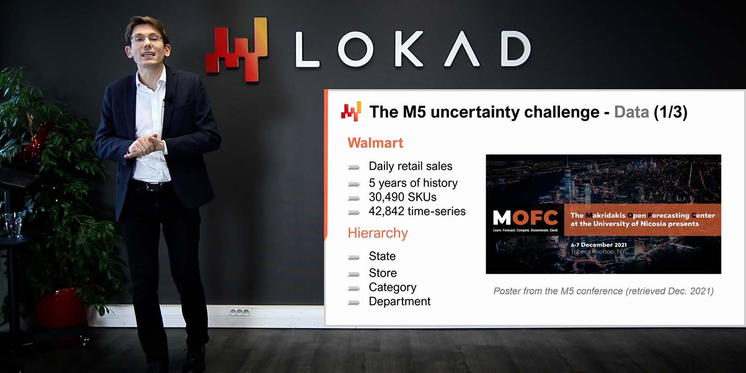
Finally, in the first lecture of this fifth chapter, we have seen a simple, some would even say simplistic, model that achieved state-of-the-art forecasting accuracy in a worldwide forecasting competition that took place in 2020. Today, I am presenting a series of techniques that can be used to learn the parameters involved with this model that I presented in the previous lecture.

The rest of this lecture will fall broadly into two blocks, followed by a few parting thoughts. The first block is dedicated to differentiable programming. We have already touched on this topic in the fourth chapter; however, we’ll have a much closer look at it today. By the end of this lecture, you should almost be able to create your own differentiable programming implementation. I’m saying “almost” because your mileage may vary depending on the tech stack that you happen to be using. Also, differentiable programming is a minor craft of its own; it takes a bit of experience to get it working smoothly in practice.
The second block of this lecture is a walkthrough for a retail demand forecasting situation. This walkthrough is a follow-up on the previous lecture, where we presented the model that achieved number one at the M5 forecasting competition in 2020. However, in this previous presentation, we did not detail how the parameters of the model were effectively computed. This walkthrough will deliver exactly that, and we will also cover important elements such as stockouts and promotions that were left unaddressed in the previous lecture. Finally, based on all these elements, I will be discussing my views on the suitability of differentiable programming for supply chain purposes.

The Stochastic Gradient Descent (SGD) is one of the two pillars of differentiable programming. The SGD is deceptively simple, and yet it is still not fully clear why it works so well. It’s absolutely clear why it works; what is not very clear is why it works so well.
The history of the Stochastic Gradient Descent can be traced back to the 1950s, so it has quite a long history. However, this technique only graduated to mainstream recognition during the last decade with the advent of deep learning. The Stochastic Gradient Descent is deeply rooted in the mathematical optimization perspective. We have a loss function Q that we want to minimize, and we have a set of real parameters, denoted W, that represent all the possible solutions. What we want to find is the combination of parameters W that minimize the loss function Q.
The loss function Q is supposed to uphold one fundamental property: it can be additively decomposed into a series of terms. The existence of this additive decomposition makes the Stochastic Gradient Descent work at all. If your loss function cannot be decomposed additively like this, then the Stochastic Gradient Descent does not apply as a technique. In this perspective, X represents the set of all the terms that contribute to the loss function, and Qx represents a partial loss that represents the loss for one of the terms in this perspective of having the loss function as the sum of partial terms.
While the Stochastic Gradient Descent is not specific to learning situations, it fits very nicely with all learning use cases, and when I say learning, I mean learning as in machine learning use cases. Indeed, if we have a training dataset, this dataset will take the form of a list of observations, with each observation being a pair of features that represent the input of the model and labels that represent the outputs. Essentially, what we want from a learning perspective is to engineer a model that performs best on the empirical error and other things as observed from this training dataset. From a learning perspective, X would actually be the list of observations, and the parameters would be the parameters of a machine learning model that we try to optimize to best fit this dataset.
The Stochastic Gradient Descent is fundamentally an iterative process that randomly iterates through the observations, one observation at a time. We pick one observation, a small X, at a time, and for this observation, we compute a local gradient, represented as nabla of Qx. It’s just a local gradient that only applies to a term of the loss function. This is not the gradient of the complete loss function itself, but a local gradient that only applies to a term of the loss function – you can see that as a partial gradient.
A step of the Stochastic Gradient Descent consists of taking this local gradient and nudging the parameters W a little based on this partial observation of the gradient. That’s exactly what is happening here, with W being updated with W minus eta times nabla QxW. This is simply saying, in a very concise form, to nudge the W parameter in the direction of the very local gradient as obtained with X, where X is just one of the observations of your dataset, if we are tackling a problem from a learning perspective. Then, we proceed at random, applying this local gradient and iterating.
Intuitively, the Stochastic Gradient Descent works very well because it displays a trade-off between faster iteration and noisier gradients, all the way to more granular and thus faster iteration. The essence of the Stochastic Gradient Descent is that we don’t care about having very imperfect measurements for our gradients as long as we can get those imperfect measurements super fast. If we can displace the trade-off all the way toward faster iteration, even at the expense of noisier gradients, let’s do it. That’s why the Stochastic Gradient Descent is so effective in minimizing the amount of computing resources needed to achieve a certain quality of solution for the parameter W.
Finally, we have the eta variable, which is referred to as the learning rate. In practice, the learning rate is not a constant; this variable varies while the Stochastic Gradient Descent is in progress. At Lokad, we use the Adam algorithm to control the evolution of this eta parameter for the learning rate. Adam is a method published in 2014, and it is very popular in machine learning circles whenever the Stochastic Gradient Descent is involved.

The second pillar for differentiable programming is automatic differentiation. We have already seen this concept in a previous lecture. Let’s revisit this concept by looking at a piece of code. This code is written in Envision, a domain-specific programming language engineered by Lokad for the purpose of predictive optimization of supply chains. I am choosing Envision because, as you will see, the examples are much more concise and hopefully much clearer as well, compared to alternative presentations if I were to use Python, Java, or C#. However, I would like to point out that even if I am using Envision, there is no secret sauce involved. You could entirely re-implement all these examples in other programming languages. It would most likely multiply the number of lines of code by a factor of 10, but in the grand scheme of things, this is a detail. Here, for a lecture, Envision gives us a very clear and concise presentation.
Let’s see how differentiable programming can be used to address a linear regression. This is a toy problem; we don’t need differentiable programming to do linear regression. The goal is merely to gain familiarity with the differentiable programming syntax. From lines 1 to 6, we are declaring the table T, which represents the observation table. When I say observation table, just remember the Stochastic Gradient Descent set that was named X. This is exactly the same thing. This table has two columns, one feature denoted X and one label denoted Y. What we want is to take X as input and be able to predict Y with a linear model, or more precisely, an affine model. Obviously, we have only four data points in this table T. This is a ridiculously small dataset; it’s just for the sake of clarity of the exposition.
At line 8, we introduce the autodiff block. The autodiff block can be seen as a loop in Envision. It’s a loop that iterates over a table, in this case, the table T. These iterations reflect the steps of the Stochastic Gradient Descent. Thus, what happens when the execution of Envision enters this autodiff block is that we have a series of repeated executions where we pick lines from the observation table and then apply steps of the Stochastic Gradient Descent. To do that, we need the gradients.
Where do the gradients come from? Here, we have written a program, a small expression of our model, Ax + B. We introduce the loss function, which is the mean squared error. We want to have the gradient. For a situation as simple as this one, we could write the gradient manually. However, automatic differentiation is a technique that lets you compile a program in two forms: the first form is the forward execution of the program, and the second form is the reverse form of execution that computes the gradients associated with all the parameters present in the program.
At lines 9 and 10, we have the declaration of two parameters, A and B, with the keyword “auto” that tells Envision to do an automatic initialization for the values of these two parameters. A and B are scalar values. The automatic differentiation happens for all the programs that are contained in this autodiff block. Essentially, it is a technique at the compiler level to compile this program twice: once for the forward pass and a second time for a program that will provide the values of the gradients. The beauty of the automatic differentiation technique is that it guarantees that the amount of CPU needed to compute the regular program is aligned with the amount of CPU needed to compute the gradient when you do the reverse pass. That’s a very important property. Finally, at line 14, we print the parameters that we have just learned with the autodiff block above.

Differentiable programming really shines as a programming paradigm. It is possible to compose an arbitrarily complex program and obtain the automated differentiation of this program. This program may include branches and function calls, for example. This code example revisits the pinball loss function that we introduced in the previous lecture. The pinball loss function can be used to derive quantile estimates when we observe deviations from an empirical probability distribution. If you minimize the mean squared error with your estimate, you get an estimate of the mean of your empirical distribution. If you minimize the pinball loss function, you get an estimate of a quantile target. If you shoot for a 90th quantile, it means that it’s the value in your probability distribution where the future value to be observed has a 90% chance to be below your estimate if you have a 90th target or a 10% chance to be above. This is reminiscent of the service levels analysis that exists in supply chain.
At lines 1 and 2, we are introducing an observation table populated with deviations randomly sampled from a Poisson distribution. The Poisson distribution values are sampled with a mean of 3, and we get 10,000 deviations. At lines 4 and 5, we roll out our bespoke implementation of the pinball loss function. This implementation is almost identical to the code that I introduced in the previous lecture. However, the keyword “autodiff” is now added to the declaration of the function. This keyword, when attached to the declaration of the function, ensures that the Envision compiler can automatically differentiate this function. While, in theory, automatic differentiation can be applied to any program, in practice, there are plenty of programs that don’t make sense to be differentiated or many functions where it would not make sense. For example, consider a function that takes two text values and concatenates them. From an automatic differentiation perspective, it doesn’t make sense to apply automatic differentiation to this sort of operation. Automatic differentiation requires numbers to be present in the input and output for the functions that you are trying to differentiate.
At lines 7 to 9, we have the autodiff block, which computes the target quantile estimate for the empirical distribution received through the observation table. Under the hood, it is actually a Poisson distribution. The quantile estimate is declared as a parameter named “quantile” at line 8, and at line 9, we make a function call to our own implementation of the pinball loss function. The quantile target is set as 0.5, so we are actually looking for a median estimate of the distribution. Finally, at line 11, we print the results for the value that we have learned through the execution of the autodiff block. This piece of code illustrates how a program that we are going to automatically differentiate can include both a function call and a branch, and all of that can happen completely automatically.

I have said that the autodiff blocks can be interpreted as a loop that performs a series of stochastic gradient descent (SGD) steps over the observation table, picking one line from this observation table at a time. However, I have remained quite elusive about the stopping condition for this situation. When does the stochastic gradient descent stop in Envision? By default, the stochastic gradient descent stops after 10 epochs. An epoch, in machine learning terminology, represents a full pass through the observation table. At line 7, an attribute named “epochs” can be attached to the autodiff blocks. This attribute is optional; by default, the value is 10, but if you specify this attribute, you can pick a different count. Here, we are specifying 100 epochs. Keep in mind that the total time for the calculation is nearly strictly linear to the number of epochs. Thus, if you have twice as many epochs, the computation time will last twice as long.
Still, at line 7, we are also introducing a second attribute named “learning_rate.” This attribute is also optional, and by default, it has the value 0.01, attached to the autodiff block. This learning rate is a factor used to initialize the Adam algorithm that controls the evolution of the learning rate. This is the eta parameter that we have seen in the step of stochastic gradient descent. It controls the Adam algorithm. Essentially, this is a parameter that you don’t frequently need to touch, but sometimes adjusting this parameter can save a significant portion of the processing power. It is not unexpected that by fine-tuning this learning rate, you can save 20% or so of the total computation time for your stochastic gradient descent.

The initialization of the parameters being learned in the autodiff block also requires closer examination. So far, we have used the keyword “auto,” and in Envision, this simply means that Envision will initialize the parameter by randomly drawing a value from a Gaussian distribution of mean 1 and standard deviation 0.1. This initialization diverges from the usual practice in deep learning, where the parameters are randomly initialized with Gaussians centered around zero. The reason why Lokad took this different approach will become clearer later on in this lecture when we proceed with an actual retail demand forecasting situation.
In Envision, it is possible to override and control the initialization of the parameters. The parameter “quantile,” for example, is declared at line 9 but doesn’t need to be initialized. Indeed, at line 7, just above the autodiff block, we have a variable “quantile” that is assigned the value 4.2, and thus the variable is already initialized with a given value. There is no need for automatic initialization anymore. It is also possible to enforce a range of allowed values for the parameters, and this is done with the keyword “in” at line 9. Essentially, we are defining that “quantile” should be between 1 and 10, inclusive. With those boundaries in place, if there is an update obtained from the Adam algorithm that would nudge the parameter value outside the acceptable range, we cap the change from Adam so that it stays within this range. In addition, we also set to zero the momentum values that are typically attached to the Adam algorithm under the hood. Enforcing parameter boundaries diverges from the classic deep learning practice; however, the benefits of this feature will become evident once we start discussing an actual retail demand forecasting example.

Differentiable programming relies heavily on stochastic gradient descent. The stochastic angle is literally what makes the descent work very fast. It is a double-edged sword; the noise obtained through the partial losses is not just a bug, but also a feature. By having a little bit of noise, the descent can avoid remaining stuck in zones with very flat gradients. So, having this noisy gradient not only makes the iteration much faster but also helps nudging the iteration to get out of areas where the gradient is very flat and causes the descent to slow down. However, one thing to keep in mind is that when stochastic gradient descent is used, the sum of the gradient is not the gradient of the sum. As a result, stochastic gradient descent comes with minor statistical biases, especially when tail distributions are concerned. However, when these concerns arise, it is relatively straightforward to duct-tape the numerical recipes, even if the theory remains a bit muddy.
Differentiable programming (DP) should not be confused with an arbitrary mathematical optimization solver. The gradient must flow through the program for differentiable programming to work at all. Differentiable programming can work with arbitrarily complex programs, but those programs have to be engineered with differentiable programming in mind. Also, differentiable programming is a culture; it’s a set of tips and tricks that play well with stochastic gradient descent. All things considered, differentiable programming is on the easy side of the machine learning spectrum. It is very approachable as a technique. Nevertheless, it takes a bit of craftsmanship to master this paradigm and operate it smoothly in production.

We are now ready to embark on the second block of this lecture: the walkthrough. We will have a walkthrough for our retail demand forecasting task. This modeling exercise is aligned with the forecasting challenge that we presented in the previous lecture. In brief, we want to forecast the daily demand at the SKU level in a retail network. An SKU, or stock-keeping unit, is technically the Cartesian product between products and stores, filtered along the entries of the assortment. For example, if we have 100 stores and 10,000 products, and if every single product is present in every store, we end up with 1 million SKUs.
There are tools to transform a deterministic estimate into a probabilistic one. We have seen one of those tools in the previous lecture through the ESSM technique. We will revisit this specific concern—turning estimates into probabilistic estimates—in greater detail in the next lecture. However, today, we are only concerned with estimating averages, and all other types of estimates (quantiles, probabilistic) will come later as natural extensions of the core example that I will present today. In this walkthrough, we are going to learn the parameters of a simple demand forecasting model. The simplicity of this model is deceptive because this class of model does achieve state-of-the-art forecasting, as illustrated in the M5 forecasting competition in 2020.

For our parametric demand model, let’s introduce a single parameter for every single SKU. This is an absolutely simplistic form of model; the demand is modeled as a constant for each SKU. However, it is not the same constant for every SKU. Once we have this constant daily average, it’s going to be the same value for all the days of the entire life cycle of the SKU.
Let’s have a look at how it’s done with differentiable programming. From lines 1 to 4, we are introducing the mock data block. In practice, this model and all its variants would depend on inputs obtained from the business systems: the ERP, WMS, TMS, etc. Presenting a lecture where I would be plugging a mathematical model into a realistic representation of data, as it is obtained from the ERP, would introduce tons of accidental complications that are irrelevant for the present topic of the lecture. So, what I’m doing here is introducing a block of mock data that is not even pretending to be realistic in any way, or the sort of data that you can observe in an actual retail situation. The only goal of this mock data is to introduce the tables and the relationships within the tables, and to make sure that the code example given is complete, can be compiled, and can be run. All the code examples you’ve seen so far are completely standalone; there are no hidden bits before or after. The sole purpose of the mock data block is to make sure that we have a standalone piece of code.
In every example in this walkthrough, we start with this mock data block. At line 1, we introduce the date table with “dates” as its primary key. Here, we have a date range that is basically two years and one month. Then, at line 2, we introduce the SKUs table, which is the list of SKUs. In this minimalistic example, we have just three SKUs. In a real retail situation for a sizable retail network, we would have millions, if not tens of millions, of SKUs. But here, for the sake of the example, I take a very small number. At line 3, we have the table “T,” which is a Cartesian product between the SKUs and the date. Essentially, what you get through this table “T” is a matrix where you have every single SKU and every single day. It has two dimensions.
At line 6, we introduce our actual autodiff block. The observation table is the SKUs table, and the stochastic gradient descent here will be picking one SKU at a time. At line 7, we introduce the “level,” which will be our sole parameter. It is a vector parameter, and so far, in our autodiff blocks, we have only introduced scalar parameters. The previous parameters were just a number; here, “SKU.level” is actually a vector. It’s a vector that has one value per SKU, and that’s literally our constant demand modeled at the SKU level. We specify a range, and we’ll see why it matters in a minute. It has to be at least 0.01, and we put 1,000 as the daily average demand’s upper bound for this parameter. This parameter is automatically initialized with a value that is close to one, which is a reasonable starting point. In this model, what we have is just one degree of freedom per SKU. Finally, at lines 8 and 9, we are actually implementing the model per se. At line 8, we are computing “dot.delta,” which is the demand as predicted by the model minus the observed, which is “T.sold.” The model is just a single term, a constant, and then we have the observation, which is “T.sold.”
To understand what is going on here, we have some broadcasting behaviors happening. The table “T” is a cross table between SKU and date. The autodiff block is an iteration that iterates over the lines of the observation table. At line 9, we are within the autodiff block, so we have picked a line for the SKU table. The value “SKUs.level” is not a vector here; it’s just a scalar, just one value because we have picked only one line of the observation table. Then “T.sold” is not a matrix anymore because we have already picked one SKU. What remains is that “T.sold” is actually a vector, a vector that has the dimension equal to date. When we do this subtraction, “SKUs.level - T.sold,” we get a vector that is aligned with the date table, and we assign it to “D.delta,” which is a vector with one line per day, two years and one month. Finally, at line 9, we are computing the loss function, which is just the mean square error. This model is super simplistic. Let’s see what can be done about calendar patterns.

Parameter sharing is probably one of the simplest and most useful differentiable programming techniques. A parameter is said to be shared if it contributes to multiple observation lines. By sharing parameters across observations, we can stabilize the gradient descent and mitigate overfitting problems. Let’s consider the day of the week pattern. We could introduce seven parameters that represent the various weights for every single SKU. So far, one SKU has only one parameter, which is just the constant demand. If we want to enrich this perception of the demand, we could say that every single day of the week comes with its own weight, and since we have seven days of the week, we can have seven weights and apply those weights multiplicatively.
However, it is unlikely for every single SKU to have its own unique day of the week pattern. The reality is that it’s much more reasonable to assume that there exists a category or some kind of hierarchy, like a product family, product category, product subcategory, or even a department in the store that correctly captures this day of the week pattern. The idea is that we don’t want to introduce seven parameters per SKU; what we want is to introduce seven parameters per category, the sort of grouping level where we assume there is a homogeneous behavior in terms of day of the week patterns.
If we decide to introduce those seven parameters with a multiplicative effect over the level, this is exactly the approach that was taken in the previous lecture for this model, which ended up number one at the SKU level in the M5 competition. We have a level and a multiplicative effect with the day of the week pattern.
In the code, in lines 1 to 5, we have the block of mock data just as previously, and we introduce an extra table named “category.” This table is a grouping table of the SKUs, and conceptually, for every single line in the SKU table, there is one and only one line that matches in the category table. In the Envision language, we say that the category is upstream of the table SKUs. Line 7 introduces the day of the week table. This table is instrumental, and we introduce it with a specific shape that reflects the cyclical pattern we want to capture. At line 7, we create the day of the week table by aggregating dates according to their value modulo seven. We are creating a table that will have exactly seven lines, and those seven lines will represent each of the seven days of the week. For every single line in the date table, each line in the database has one and only one counterpart in the day of the week table. Thus, following the Envision language, the day of the week table is upstream of the table “date.”
Now we have the table “CD,” which is a Cartesian product between category and day of the week. In terms of the number of lines, this table will have as many lines as there are categories times seven because the day of the week has seven lines. At line 12, we introduce a new parameter named “CD.DOW” (DOW stands for day of the week), which is another vector parameter belonging to the table CD. In terms of degrees of freedom, we will have exactly seven parameter values times the number of categories, which is what we seek. We want a model that is able to capture this day of the week pattern but with only one pattern per category, not one pattern per SKU.
We declare this parameter, and we use the “in” keyword to specify that the value for “CD.DOW” should be between 0.1 and 100. At line 13, we write the demand as expressed by the model. The demand is “SKUs.level * CD.DOW,” representing the demand. We have the demand minus the observed “T.sold,” and that gives us a delta. Then we compute the mean square error.
At line 13, we have quite a bit of broadcasting magic going on. “CD.DOW” is a cross table between category and day of the week. Because we are within the autodiff block, the table CD is a cross table between category and day of the week. Since we are within the autodiff block, the block is iterating over the SKUs table. Essentially, when we pick one SKU, we have effectively picked one category, as the category table is upstream. This means that CD.DOW is not a matrix anymore, but rather a vector of dimension seven. However, it is upstream of the table “date,” so those seven lines can be broadcast in the date table. There is only one way to do this broadcast because each line of the day of the week table has an affinity with specific lines of the date table. We have a double broadcast going on, and in the end, we obtain a demand that is a series of values that is cyclical at the day of the week level for the SKU. That’s our model at this point, and the rest of the loss function remains unchanged.
We see a very elegant way to approach cyclicities by combining the broadcasting behaviors obtained from the relational nature of Envision with its differentiable programming capabilities. We can express calendar cyclicities in just three lines of code. This approach works well even if we are dealing with very sparse data. It would work just fine even if we were looking at products that sold only one unit per month on average. In such cases, the wise approach would be to have a category that includes dozens, if not hundreds of products. This technique can also be used to reflect other cyclical patterns, such as the month of the year or the day of the month.
The model introduced in the previous lecture, which achieved state-of-the-art results at the M5 competition, was a multiplicative combination of three cyclicities: day of the week, month of the year, and day of the month. All these patterns were chained as a multiplication. Implementing the two other variants is left to the attentive audience, but it is just a matter of a couple of lines of code per cyclical pattern, making it very concise.

In the previous lecture, we introduced a sales forecasting model. However, it is not the sales that interest us, but the demand. We should not confuse zero sales with zero demand. If there was no stock left for the customer to buy in the store on a given day, the loss masking technique is used at Lokad to cope with stockouts. This is the simplest technique used to cope with stockouts, but it’s not the only one. As far as I know, we have at least two other techniques that are used in production, each with their own pros and cons. Those other techniques won’t be covered today, but they will be addressed in later lectures.
Returning to the code example, lines 1 to 3 remain untouched. Let’s examine what follows. At line 6, we are enriching the mock data with the in-stock boolean flag. For every single SKU and every single day, we have a boolean value that indicates whether there was a stockout at the end of the day for the store. At line 15, we are modifying the loss function to exclude, by zeroing them, the days where a stockout was observed at the end of the day. By zeroing those days, we are ensuring that no gradient is backpropagated in situations that present a bias due to the occurrence of the stockout.
The most puzzling aspect of the loss masking technique is that it does not even change the model. Indeed, if we look at the model expressed at line 14, it is exactly the same; it has not been touched. It is only the loss function itself that is modified. This technique may be simple, but it profoundly diverges from a model-centric perspective. It is, at its core, a modeling-centric technique. We are making the situation better by acknowledging the bias caused by stockouts, reflecting this in our modeling efforts. However, we are doing this by changing the accuracy metric, not the model itself. In other words, we are changing the loss that we optimize, making this model non-comparable with other models in terms of pure numerical error.
For a situation like Walmart, as discussed in the previous lecture, the loss masking technique is adequate for most products. As a rule of thumb, this technique works well if the demand is not so sparse that you only have one unit in stock most of the time. Additionally, you should avoid products where stockouts are very frequent because it is the explicit strategy of the retailer to end up with a stockout at the end of the day. This typically happens for some ultra-fresh products where the retailer is aiming for an out-of-stock situation by the end of the day. Alternative techniques remedy these limitations, but we do not have time to cover them today.

Promotions are an important aspect of retail. More generally, there are plenty of ways for the retailer to influence and shape demand, such as pricing or moving goods to a gondola. The variables that provide extra information for predictive purposes are typically referred to as covariates in supply chain circles. There is a lot of wishful thinking about complex covariates like weather data or social media data. However, before delving into advanced topics, we need to address the elephant in the room, such as pricing information, which obviously has a significant impact on the demand that will be observed. Thus, at line 7 in this code example, we introduce for every single day at line 14, “category.ed”, where “ed” stands for elasticity of demand. This is a shared vector parameter with one degree of freedom per category, intended as a representation of the elasticity of demand. At line 16, we introduce an exponential form of price elasticity as the exponential of (-category.ed * t.price). Intuitively, with this form, when the price increases, the demand converges rapidly to zero due to the presence of the exponential function. Conversely, when the price converges to zero, the demand explosively increases.
This exponential form of pricing response is simplistic, and sharing the parameters ensures a high degree of numerical stability even with this exponential function in the model. In real-world settings, especially for situations like Walmart, we would have several pricing information, such as discounts, the delta compared to the normal price, covariates representing marketing pushes executed by the supplier, or categorical variables that introduce things like gondolas. With differentiable programming, it is straightforward to craft arbitrarily complex price responses that closely fit the situation. Integrating covariates of almost any kind is very straightforward with differentiable programming.

Slow movers are a fact of life in retail and many other verticals. The model introduced so far has one parameter, one degree of freedom per SKU, with more if you count the shared parameters. However, this might already be too much, especially for SKUs that only rotate once a year or just a few times a year. In such situations, we cannot even afford one degree of freedom per SKU, so the solution is to rely solely on shared parameters and remove all parameters with degrees of freedom at the SKU level.
At lines 2 and 4, we introduce two tables named “products” and “stores”, and the table “SKUs” is constructed as a filtered subtable of the Cartesian product between products and stores, which is the very definition of assortment. At lines 15 and 16, we introduced two shared vector parameters: one level with an affinity with the products table and another level that has an affinity with the store tables. These parameters are also defined within a specific range, from 0.01 to 100, which is the max value.
Now, at line 18, the level per SKU is composed as the multiplication of the product level and the store level. The rest of the script remains unchanged. So, how does it work? At line 19, SKU.level is a scalar. We have the autodesk block that iterates over the SKUs table, which is the observation table. Thus, SKUs.level at line 18 is just a scalar value. Then we have products.level. Since the products table is upstream of the SKUs table, for every single SKU, there is one and only one product table. Thus, products.level is just a scalar number. The same applies to the stores table, which is also upstream of the SKUs table. At line 18, there is only one store attached to this specific SKU. Therefore, what we have is the multiplication of two scalar values, which gives us the SKU.level. The rest of the model remains unchanged.
These techniques put a completely new light on the claim that sometimes there is not enough data or that sometimes the data is too sparse. Indeed, from the differentiable perspective, those claims don’t even really make sense. There is no such thing as too little data or the data being too sparse, at least not in absolute terms. There are just models that can be modified toward sparsity and possibly toward extreme sparsity. The imposed structure is like guiding rails that make the learning process not only possible but numerically stable.
Compared to other machine learning techniques that try to let the machine learning model discover all the patterns ex nihilo, this structured approach establishes the very structure that we have to learn. Thus, the statistical mechanism at play here has limited freedom in what it is to learn. Consequently, in terms of data efficiency, it can be incredibly efficient. Naturally, all of this relies on the fact that we have chosen the right structure.
As you can see, doing experiments is very straightforward. We are already doing something very complicated, and in less than 50 lines, we could deal with a fairly complex Walmart-like situation. This is quite an achievement. There is a bit of an empirical process, but the reality is that it’s not that much. We are talking about a few dozen lines. Keep in mind that an ERP like the one that is running a company, a large retail network, has typically a thousand tables and 100 fields per table. So, clearly, the complexity of the business systems is absolutely gigantic compared to the complexity of this structured predictive model. If we have to spend a little bit of time iterating, it’s almost nothing.
Moreover, as demonstrated in the M5 forecasting competition, the reality is that supply chain practitioners already know the patterns. When the M5 team used three calendar patterns, which were day of the week, month of the year, and day of the month, all of these patterns were self-evident to any experienced supply chain practitioner. The reality in supply chain is that we are not trying to discover some hidden pattern. The fact that, for example, if you massively drop the price, it’s going to massively increase the demand, is not going to surprise anyone. The only question that is left is what is exactly the magnitude of the effect and what is the exact shape of the response. These are relatively technical details, and if you allow yourself the opportunity to do a little bit of experiments, you can address these problems relatively easily.

As a last step of this walkthrough, I would like to point out a minor quirk of differentiable programming. Differentiable programming should not be confused with a generic mathematical optimization solver. We need to keep in mind that there is a gradient descent going on. More specifically, the algorithm used to optimize and update the parameters has a maximum descent speed that is equal to the learning rate that comes with the ADAM algorithm. In Envision, the default learning rate is 0.01.
If we look at the code, at line 4, we introduced an initialization where the quantities being sold are sampled from a Poisson distribution with a mean of 50. If we want to learn a level, technically, we would need to have a level that would be of the order of 50. However, when we do an automatic initialization of the parameter, we start with a value that is around one, and we can only go in increments that are 0.01. It would take something like 5,000 epochs to actually reach this value of 50. Since we have a non-shared parameter, SKU.level, this parameter per epoch is only touched once. Thus, we would need 5,000 epochs, which would needlessly slow down the computation.
We could increase the learning rate to speed up the descent, which would be one solution. However, I would not advise inflating the learning rate, as this is typically not the right way to approach the problem. In a real situation, we would have shared parameters in addition to this non-shared parameter. Those shared parameters are going to be touched by the stochastic gradient descent many times throughout each epoch. If you vastly increase the learning rate, you risk creating numerical instabilities for your shared parameters. You could increase the movement speed of the SKU level but create numerical stability problems for the other parameters.
A better technique would be to use a rescaling trick and wrap the parameter into an exponential function, which is exactly what is done at line 8. With this wrapper, we can now reach parameter values for the level that can be either very low or very high with a much smaller number of epochs. This quirk is basically the only quirk that I would need to introduce to have a realistic example for this walkthrough of retail demand forecasting situation. All things considered, it is a minor quirk. Nevertheless, it’s a reminder that differentiable programming requires paying attention to the flow of gradients. Differentiable programming offers a fluid design experience overall, but it’s not magic.

A few parting thoughts: structured models do achieve state-of-the-art forecasting accuracy. This point was extensively made in the previous lecture. However, based on the elements presented today, I would argue that accuracy is not even the decisive factor in favor of differentiable programming with a structured parametric model. What we get is understanding; we do not only get a piece of software that is capable of making predictions, but we also get direct insights into the very patterns that we are trying to capture. For example, the model introduced today would directly give us a demand forecast that comes with explicit day-of-the-week weights and an explicit elasticity of the demand. If we were to extend this demand, for example, to introduce an uplift associated with Black Friday, a quasi-seasonal event that doesn’t happen at the same time every single year, we could do that. We would just add a factor, and then we would have an estimate for the Black Friday uplift in isolation of all the other patterns, such as the day-of-the-week pattern. This is of prime interest.
What we get through the structured approach is understanding, and it is a lot more than just the raw model. For example, if we end up with a negative elasticity, a situation where the model tells you that when you increase the price, you increase the demand, in a Walmart-like situation, this is a very dubious result. Most likely, it reflects that your model implementation is flawed, or that there are deep problems going on. No matter what the accuracy metric tells you, if you end up in a Walmart situation with something that tells you that by making a product more expensive, people buy more, you should really question your entire data pipeline because most likely, there is something very wrong. That’s what understanding is about.
Also, the model is open to change. Differentiable programming is incredibly expressive. The model that we have is just one iteration in a journey. If the market is transformed or if the company itself is transformed, we can rest assured that the model that we have will be able to capture this evolution naturally. There is no such thing as an automatic evolution; it will take effort from a supply chain scientist to capture this evolution. However, this effort can be expected to be relatively minimal. It boils down to the fact that if you have a very small, tidy model, then when you need to revisit this model later on to adjust its structure, it’s going to be a relatively small task compared to a situation where your model would be a beast of engineering.
When engineered carefully, models produced with differentiable programming are very stable. The stability boils down to the choice of structure. Stability is not a given for any program that you optimize through differentiable programming; it is the sort of thing that you get when you have a very clear structure where the parameters have a specific semantic. For example, if you have a model where, whenever you retrain your model, you end up with completely different weights for the day of the week, then the reality in your business is not changing that fast. If you run your model twice, you should end up with values for the day of the week that are fairly stable. If it’s not the case, then there is something very wrong in the way that you’ve modeled your demand. Thus, if you make a wise choice for the structure of your model, you can end up with incredibly stable numerical results. By doing that, we avoid pitfalls that tend to plague complex machine learning models when we try to use them in a supply chain context. Indeed, from a supply chain perspective, numerical instabilities are deadly because we have ratchet effects all over the place. If you have an estimation of the demand that fluctuates, it means that randomly you’re going to trigger a purchase order or a production order just for nothing. Once you’ve triggered your production order, you can’t decide next week that it was a mistake and you should not have done that. You’re stuck with the decision that you’ve just taken. If you have an estimator of future demand that keeps fluctuating, you will end up with inflated replenishment and inflated production orders. This issue can be solved by ensuring stability, which is a matter of design.
One of the biggest hurdles of getting machine learning in production is trust. When you operate over millions of euros or dollars, understanding what is going on in your numerical recipe is critical. Supply chain mistakes can be exceedingly costly, and there are plenty of examples of supply chain disasters driven by poor application of badly understood algorithms. While differentiable programming is very powerful, the models that can be engineered are incredibly simple. These models could actually be run in an Excel spreadsheet, as they are typically straightforward multiplicative models with branches and functions. The only aspect that could not run in an Excel spreadsheet is the automatic differentiation, and obviously, if you have millions of SKUs, don’t attempt to do that in a spreadsheet. However, simplicity-wise, it is very much compatible with something that you would put in a spreadsheet. This simplicity goes a long way in establishing trust and bringing machine learning into production, instead of keeping them as fancy prototypes that people never quite manage to trust completely.
Finally, when we put all these properties together, we get a very accurate piece of technology. This angle was discussed in the very first chapter of this series of lectures. We want to turn all the efforts invested into supply chain into capitalistic investments, as opposed to treating supply chain experts and practitioners as consumables that need to do the same things over and over. With this approach, we can treat all these efforts as investments that will generate and keep generating return on investment over time. Differentiable programming plays very well with this capitalistic perspective for supply chain.

In the second chapter, we introduced an important lecture titled “Experimental Optimization,” which provided one possible answer to the simple yet fundamental question: What does it mean to actually improve or do better in a supply chain? The differentiable programming perspective provides a very specific insight on many struggles faced by supply chain practitioners. Enterprise software vendors frequently blame bad data for their supply chain failures. However, I believe this is just the wrong way to look at the problem. The data is just what it is. Your ERP has never been engineered for data science, but it has been operating smoothly for years, if not decades, and people in the company manage to run the supply chain nevertheless. Even if your ERP that captures data about your supply chain isn’t perfect, it’s okay. If you expect that perfect data will be made available, this is just wishful thinking. We are talking about supply chains; the world is very complex, so systems are imperfect. Realistically, you don’t have one business system; you have like half a dozen, and they are not completely consistent with one another. This is just a fact of life. However, when enterprise vendors blame bad data, the reality is that a very specific forecasting model is used by the vendor, and this model has been engineered with a specific set of assumptions about the company. The problem is that if your company happens to violate any of those assumptions, the technology falls apart completely. In this situation, you have a forecasting model that comes with unreasonable assumptions, you feed the data, it’s not perfect, and thus the technology falls apart. It is completely unreasonable to say that the company is at fault. The technology at fault is the one being pushed by the vendor that makes completely unrealistic assumptions about what data can even be in a supply chain context.
I haven’t presented any benchmark for any accuracy metric today. However, my proposition is that those accuracy metrics are mostly inconsequential. A predictive model is a tool to drive decisions. What matters is whether those decisions—what to buy, what to produce, whether to move your price up or down—are good or bad. Bad decisions can be traced back to the predictive model, that is true. However, most of the time, it is not an accuracy problem. For example, we had a sales forecasting model, and we fixed the stock out angle that was not managed appropriately. However, when we fixed the stock out angle, what we did is to fix the accuracy metric itself. So, fixing the predictive model doesn’t mean improving the accuracy; very frequently, it means literally revisiting the very problem and perspective in which you operate, and thus modifying the accuracy metric or something even more profound. The problem with the classic perspective is that it assumes that the accuracy metric is a worthy goal. This is not entirely the case.
Supply chains operate in a real world, and there are plenty of unexpected and even freak events. For example, you can have an obstruction of the Suez Canal due to a ship; this is a completely freak event. In such a situation, it would immediately invalidate all the lead-time forecasting models in existence that were looking at this portion of the world. Obviously, this was something that had not really happened before, so we can’t really backtest anything in such a situation. However, even if we have this completely exceptional situation with a ship blocking the Suez Canal, we can still fix the model, at the very least if we have this kind of white-box approach that I’m putting forward today. This fix is going to involve a degree of guesswork, which is okay. It’s better to be approximately right rather than exactly wrong. For example, if we’re looking at the Suez Canal being blocked, you can just say, “let’s add one month to the lead time for all the supplies that were supposed to go through this route.” This is very approximate, but it’s better to assume that there will be no delay at all, although you already have the information. Additionally, change frequently comes from within. For example, let’s consider a retail network that has one old distribution center and a new distribution center supplying a few dozen stores. Let’s say that there is a migration going on, where essentially the supplies for the stores are being migrated from the old distribution center to the new one. This situation happens almost only once in the history of this specific retailer, and it can’t really be back-tested. Yet, with an approach like differentiable programming, it is completely straightforward to implement a model that would fit this gradual migration.

In conclusion, differentiable programming is a technology that gives us an approach to structure our insights about the future. Differentiable programming lets us shape, quite literally, the way we look at the future. Differentiable programming is on the perception side of this picture. Based on this perception, we can take better decisions for supply chains, and those decisions drive the actions that are on the other side of the picture. One of the biggest misunderstandings of the mainstream supply chain theory is that you can treat perception and action in isolation as strictly isolated components. This takes the form, for example, of having one team in charge of planning (that’s perception) and one independent team in charge of replenishment (that’s action).
However, the perception-action feedback loop is very important; it is of primary importance. This is literally the very mechanism that guides you towards a correct form of perception. If you don’t have this feedback loop, it’s not even clear if you’re looking at the right thing, or if the thing you’re looking at is really what you think it is. You need this feedback mechanism, and it is through this feedback loop that you can actually steer your models toward a correct quantitative assessment of the future that is relevant for the course of action for your supply chain. The mainstream supply chain approaches are dismissing this case almost entirely because, essentially, I believe they are stuck with a very rigid form of forecasting. This model-centric form of forecasting can be an old model, like the Holt-Winters forecasting model, or a recent one like Facebook Prophet. The situation is the same: if you’re stuck with one forecasting model, then all the feedback that you can get from the action side of the picture is moot because you cannot do anything about this feedback except ignore it entirely.
If you’re stuck with a given forecasting model, you can’t reformat or restructure your model as you get information from the action side. On the other hand, differentiable programming, with its structured modeling approach, gives you a completely different paradigm. The predictive model is completely disposable—all of it. If the feedback that you get from your action calls for radical changes in your predictive perspective, then simply implement those radical changes. There is no specific attachment to a given iteration of the model. Keeping the model very simple goes a long way in making sure that once in production, you preserve the option to keep changing this model. Because, again, if what you’ve engineered is like a beast, an engineering monster, then once you’re in production, it becomes incredibly difficult to change it. One of the key aspects is that if you want to be able to keep changing, you need to have a model that is very parsimonious in terms of lines of code and internal complexity. This is where differentiable programming shines. It’s not about achieving higher accuracy; it’s about achieving higher relevance. Without relevance, all the accuracy metrics are completely moot. Differentiable programming and structured modeling give you the journey to achieve relevance and then maintain relevance over time.

This will conclude the lecture for today. Next time, on the second of March, same time of the day, 3 PM Paris time, I will be presenting probabilistic modeling for supply chain. We’ll have a closer look at the technical implications of looking at all the possible futures instead of merely picking one future and declaring it the right one. Indeed, looking at all the possible futures is very important if you want your supply chain to be resilient effectively against risk. If you just pick one future, it is a recipe to end up with something that is incredibly fragile if your forecast doesn’t happen to be perfectly correct. And guess what, the forecast is never completely correct. That’s why it’s very important to embrace the idea that you need to look at all the possible futures, and we will have a look at how to do that with modern numerical recipes.
Question: Stochastic noise is added to avoid local minima, but how is it leveraged or scaled to avoid large deviations so that gradient descent is not thrown far away from its goal?
That’s a very interesting question, and there are two parts to this answer.
First, this is why the Adam algorithm is very conservative in terms of the magnitude of the movements. The gradient is fundamentally unbounded; you can have a gradient that is worth thousands or millions. However, with Adam, the maximal step is actually upper bounded by the learning rate. So, effectively, Adam comes with a numerical recipe that literally enforces a maximal step, and hopefully, that avoids massive numerical instability.
Now, if at random, despite the fact that we have this learning rate, we could say that just out of sheer fluctuation we are going to move iteratively, one step at a time, but many times in a direction that is incorrect, this is a possibility. That’s why I say that the stochastic gradient descent is still not completely understood. It works incredibly well in practice, but why it works so well, and why it converges so fast, and why we don’t get more of the problems that may happen, is not completely understood, especially if you consider that the stochastic gradient descent happens in high dimensions. So typically, you have literally tens, if not hundreds, of parameters that are being touched at every step. The sort of intuition that you can have in two or three dimensions is very misleading; things behave very differently when you’re looking at higher dimensions.
So, the bottom line for this question: it’s very relevant. There is one part where it’s the Adam magic of being very conservative with the scale of your gradient steps, and the other part, which is poorly understood but yet in practice works very well. By the way, I believe the fact that the stochastic gradient descent is not completely intuitive is also the reason why for almost 70 years this technique was known but not recognized as effective. For almost 70 years, people knew that it existed, but they were highly skeptical. It took the massive success of deep learning for the community to recognize and acknowledge that it’s actually working very well, even if we don’t really understand why.
Question: How does one understand when a certain pattern is weak and should therefore be removed from the model?
Again, a very good question. There is no strict criteria; it’s literally a judgment call from the supply chain scientist. The reason is that if the pattern you introduce gives you minimal benefits, but in terms of modeling it is only two lines of code and the impact in terms of amount of computation time is insignificant, and if you ever want to remove the pattern later on it is semi-trivial, you could say, “Well, I can just keep it. It doesn’t seem to hurt, it doesn’t do much good. I can see situations where this pattern that is weak now could actually become strong.” In terms of maintainability, that’s fine.
However, you can also see the other side of the picture where you have a pattern that doesn’t capture much, and it adds a lot of compute to the model. So it’s not free; every single time you add a parameter or logic, you’re going to inflate the amount of computing resources needed for your model, making it slower and more unwieldy. If you think this pattern that is weak could actually become strong, but in a bad way, generating instability and creating havoc in your predictive modeling, this is typically the sort of situation where you would think, “No, I should probably remove it.”
You see, it is really a matter of judgment call. Differentiable programming is a culture; you’re not on your own. You have colleagues and peers who have maybe tried different things at Lokad. This is the sort of culture that we try to cultivate. I know that it might be a bit of a disappointment compared to the all-powerful AI perspective, the idea that we could have an all-powerful artificial intelligence solving all those problems for us. But the reality is that supply chains are so complex, and our techniques of artificial intelligence are so crude that we don’t have any realistic substitute for human intelligence. When I say judgment call, I just mean that you need a healthy dose of applied, very human intelligence to the case, because all the algorithmic tricks are not even close to delivering a satisfying answer.
Nevertheless, it doesn’t mean that you can’t design some kind of tooling. That would be another topic; I will see if I will actually cover the sort of tooling that we provide at Lokad to facilitate the design. A tangential pattern would be, if we have to make a judgment call, let’s try to provide all the instrumentation so that this judgment call can be made very swiftly, minimizing the amount of pain that comes with this sort of indecision where the supply chain scientist needs to decide something about the fate of the present state of the model.
Question: What is the complexity threshold of a supply chain after which machine learning and differentiable programming bring considerably better results?
At Lokad, we typically manage to bring substantial results for companies that have a turnover of $10 million per year and over. I would say it really starts to shine if you have a company with an annual turnover of $50 million and over.
The reason is that fundamentally, you need to establish a very reliable data pipeline. You need to be able to extract all the relevant data from the ERP on a daily basis. I don’t mean that it’s going to be good data or bad data, just the data that you have can have plenty of defects. Nonetheless, it means there is quite a lot of plumbing just to be able to extract the very basic transactions on a daily basis. If the company is too small, then usually they don’t even have a dedicated IT department, and they can’t manage to have reliable daily extraction, which really compromises the results.
Now, in terms of verticals or complexity, the thing is, in most companies and most supply chains, in my opinion, they haven’t even started to optimize yet. As I said, the mainstream supply chain theory emphasizes that you should chase more accurate forecasts. Having a reduced percentage of forecasting error is a goal, and many companies, for example, would go at it by having a planning team or a forecasting team. In my opinion, all of that is not adding anything of value to the business because it is fundamentally providing very sophisticated answers to the wrong set of questions.
It might come as a surprise, but differentiable programming really shines not because it is fundamentally super powerful – it is – but it shines because it’s usually the first time that there is something that is truly relevant to the business put in place in the company. If you just want to have an example, most of what is implemented in supply chain is typically models like the safety stock model, which have absolutely zero relevance to any real-world supply chain whatsoever. For example, in the safety stock model, you assume that it’s possible to have negative lead time, meaning that you order now and you will be delivered yesterday. It doesn’t make any sense, and as a consequence, the operational results for safety stocks are usually unsatisfactory.
Differentiable programming shines by achieving relevance, not by achieving some kind of grand numerical superiority or by being better than other alternative machine learning techniques. The point is really achieving relevance in a world that is very complex, chaotic, adversarial, changing all the time, and where you have to deal with a semi-nightmarish applicative landscape that represents the data you have to process.
It seems that there are no more questions. In this case, I guess I’ll see you next month for the probabilistic modeling for the supply chain lecture.